Deriving the Dirac Delta Term in the Dipole Electric Field Formula
2025-04-20
Introduction
The inspiration for today’s post is J.D. Jackson’s "Classical Electrodynamics", which I have been dutifully plodding through for several months now. I recently started Chapter 4 which covers multipole expansions and their application to the study of dielectrics and electrostatics of macroscopic media.
In section 4.1, Jackson presented an interesting derivation of the formula for the electric field of a dipole
\mathbf{E}(\mathbf{x})=\frac{1}{4\pi\epsilon_0}\left[\frac{3\mathbf{n}(\mathbf{p}\cdot\mathbf{n})-\mathbf{p}}{|\mathbf{x}-\mathbf{x}_0|^3}-\frac{4\pi}{3}\mathbf{p}\delta(\mathbf{x}-\mathbf{x}_0)\right]
The derivation uses some very nice tricks, making it satisfying to read, and will be (according to Jackson) "useful in elucidating the basic difference between electric and magnetic dipoles."
However, in the true Jacksonian style, many important details of the derivation are omitted and considered too trivial for the consideration of the great J.D. I spent a good part of my Saturday morning working out some of these details, and I am now sharing my results with the world. I hope this post will provide some intellectual satisfaction to readers and make this derivation more understandable to anyone struggling through Jackson.
Before beginning, I must warn that this blog post will not be very accessible to people lacking background in electrodynamics and vector calculus. There are many identities and formulas used here, and deriving all of them would not make sense, given that any electrodynamics student should know them.
With those preliminaries covered, let us begin!
The Derivation
Jackson begins by considering a localized charge distribution \rho(\mathbf{x}) that leads to an electric field \mathbf{E}(\mathbf{x}) throughout space. He proposes integrating the electric field over the volume of a sphere of radius R.
We choose the origin as the center of the sphere and begin with
\int_{r<R}\mathbf{E}(\mathbf{x})\,d^3x=-\int_{r<R}\boldsymbol{\nabla}\Phi\,d^3x
Now we use the following important identity to turn our volume integral into a surface integral
\iiint_{V}\boldsymbol{\nabla} f\,dV=\iint_{\partial V}f \cdot \mathbf{n}\,dS
where \mathbf{n} is the outward unit normal to the boundary of V, \partial V.
For anyone unfamiliar with this identity, it can be easily derived using the divergence theorem – proof left as an exercise for the reader.
Use of this identity yields
\int_{r<R}\mathbf{E}(\mathbf{x})\,d^3x=-\int_{r=R}\Phi \mathbf{n}\,dA
where n is the outward directed normal to the sphere i.e. \mathbf{n}=\mathbf{x}/R
Now Jackson switched our integral over area elements to an integral over solid angle. The appropriate scale factor is
\,dA=R^2\,d\Omega
For those unfamiliar with solid angle integration, the Wikipedia article gives a decent introduction.
Using this change to solid angle integration, we find
\int_{r<R}\mathbf{E}(\mathbf{x})\,d^3x=-\int_{r=R}R^2\,d\Omega \Phi(\mathbf{x})\mathbf{n}
Now Jackson brings in the definition of electrostatic potential as a volume integral i.e.
\Phi(\mathbf{x})=\frac{1}{4\pi\epsilon_0}\int_{}\frac{\rho(\mathbf{x'})}{|\mathbf{x}-\mathbf{x'}|}\,d^3x'
Substitution of this formula gives us
\int_{r<R}\mathbf{E}(\mathbf{x})\,d^3x=-\frac{R^2}{4\pi\epsilon_0} \int_{r=R}\mathbf{n}\,d\Omega \int_{}\frac{\rho(\mathbf{x'})}{|\mathbf{x}-\mathbf{x'}|}\,d^3x'
Jackson interchanges the two integration operators (justified by Fubini’s Theorem I think? I haven’t studied analysis, if anyone has the time I’d love to see how we justify this interchange) now to get
\int_{r<R}\mathbf{E}(\mathbf{x})\,d^3x=-\frac{R^2}{4\pi\epsilon_0} \int_{}\,d^3x'\rho(\mathbf{x'}) \int_{r=R}\frac{\mathbf{n}}{|\mathbf{x}-\mathbf{x'}|}\,d\Omega
Thus far Jackson has been quite friendly – we’ve been dealing with very basic vector calculus and haven’t met anything outlandish. Here, however, all hell breaks lose.
We focus on the surface integral first.
Recall that the normal vector to the sphere can be expressed as \mathbf{n}=\mathbf{x}/R, allowing us to express the normal vector in spherical coordinates now
\mathbf{n}=\mathbf{i}\sin\theta\cos\phi+\mathbf{j}sin\theta\sin\phi+\mathbf{k}\cos\theta=\sin\theta(\mathbf{i}\cos\phi+\mathbf{j}\sin\phi)+\mathbf{k}\cos\theta
Now Jackson invites us to notice, as any normal person would (sarcasm), that the components of this vector can all be expressed as linear combinations of spherical harmonics with l=1
A quick look at a table of spherical harmonics reveals this to be true. Indeed, we can find quite easily that
\begin{split} \mathbf{n}&=\sqrt{\frac{2\pi}{3}}\biggl([-Y_{1,1}(\theta,\phi)+Y_{1,-1}(\theta,\phi)]\mathbf{i}+i[Y_{1,1}(\theta,\phi)+Y_{1,-1}(\theta,\phi)]\mathbf{j}\biggr) \\ &+\sqrt{\frac{4\pi}{3}}Y_{1,0}(\theta,\phi)\mathbf{k} \end{split}
Now, the central theme of this chapter is using spherical harmonics to find cool series expansions. So the next step is rather obvious.
We recall our expansion for \frac{1}{|\mathbf{x}-\mathbf{x'}|} in terms of spherical harmonics as
\frac{1}{|\mathbf{x}-\mathbf{x'}|}=4\pi\sum_{l=0}^{\infty}\frac{1}{2l+1}\frac{r_<^l}{r_>^{l+1}}\sum_{m=-l}^{l}Y_{lm}^*(\theta',\phi')Y_{lm}(\theta,\phi)
where r_> is the greater of r and r' and r_< is the smaller of the two.
Now we combine these two results to express the solid angle integral as
\int_{r=R}\,d\Omega\frac{\mathbf{n}}{|\mathbf{x}-\mathbf{x'}|}=4\pi\int_{r=R}\,d\Omega \mathbf{n}\sum_{l=0}^{\infty}\frac{1}{2l+1}\frac{r_<^l}{r_>^{l+1}}\sum_{m=-l}^{l}Y_{lm}^*(\theta',\phi')Y_{lm}(\theta,\phi)
Now let’s interchange the summation operators with the integration operator and take terms independent of \Omega outside of the integral.
\int_{r=R}\,d\Omega\frac{\mathbf{n}}{|\mathbf{x}-\mathbf{x'}|}=4\pi\sum_{l=0}^{\infty}\frac{r_<^l}{(2l+1)r_>^{l+1}}\sum_{m=-l}^{l}Y_{lm}^*(\theta',\phi')\int_{r=R}Y_{lm}(\theta,\phi)\mathbf{n}\,d\Omega
Now consider just this part of the expression
Y_{lm}^*(\theta',\phi')\int_{r=R}Y_{lm}(\theta,\phi)\mathbf{n}\,d\Omega
Recall our expression for \mathbf{n} in terms of spherical harmonics. Ignore the constants in that and consider its general form, giving us
\begin{split} Y_{lm}^*(\theta',\phi')\int_{r=R}Y_{lm}(\theta,\phi)\mathbf{n}\,d\Omega=\\ Y_{lm}^*(\theta',\phi')\int_{r=R}Y_{lm}(\theta,\phi) \left[a(-Y_{1,1}+Y_{1,-1}) \mathbf{i}+b(Y_{1,1}+Y_{1,-1}) \mathbf{j}+cY_{1,0} \mathbf{k}\right]\,d\Omega \end{split}
Now we must recall the orthogonality relation for spherical harmonics
\int_{r=R}Y_{lm}(\theta,\phi)Y_{l'm'}(\theta,\phi)\,d\Omega=\delta_{ll'}\delta_{mm'}
Evidently, the only nonvanishing terms here are the l=1 terms because of our orthogonality relation and the expression for \mathbf{n} in terms of Y_{1m} spherical harmonics.
Thus, we have \int_{r=R}\,d\Omega\frac{\mathbf{n}}{|\mathbf{x}-\mathbf{x'}|}=4\pi\cdot\frac{r_<}{3r_>^2}\sum_{m=-1}^{1}Y_{1m}^*(\theta',\phi')\int_{r=R}Y_{1m}(\theta,\phi)\mathbf{n}\,d\Omega
Quite a simplification! We have even more nice tricks here though.
Again consider
\sum_{m=-1}^{1}Y_{lm}^*(\theta',\phi')\int_{r=R}Y_{lm}(\theta,\phi)\mathbf{n}\,d\Omega
To make our expression for \mathbf{n} a bit less ugly, I’ll write it in a more abstract form as
\mathbf{n}=\sum_{a=1}^{3}\mathbf{e}_a\sum_{b=-1}^{1}Y_{1b}(\theta,\phi)c_{ab}
where \mathbf{e}_1=\mathbf{i},\mathbf{e}_2=\mathbf{j},\mathbf{e}_3=\mathbf{k}
Comparison with our earlier expression shows that this is essentially the same thing – just let c_{11}=-\sqrt{\frac{2\pi}{3}},c_{30}=\sqrt{\frac{4\pi}{3}} etc
Now let’s look again at \begin{split} &\sum_{m=-1}^{1}Y_{lm}^*(\theta',\phi')\int_{r=R}Y_{lm}(\theta,\phi)\mathbf{n}\,d\Omega\\ &= \sum_{m=-1}^{1}Y_{lm}^*(\theta',\phi')\int_{r=R}Y_{lm}(\theta,\phi)\sum_{a=1}^{3}\mathbf{e}_a\sum_{b=-1}^{1}Y_{1b}(\theta,\phi)c_{ab}\,d\Omega\\ &= \sum_{m=-1}^{1}Y_{lm}^*(\theta',\phi')\sum_{a=1}^{3}\mathbf{e}_a\sum_{b=-1}^{1}c_{ab}\int_{r=R}Y_{lm}(\theta,\phi)Y_{1b}(\theta,\phi)\,d\Omega\\ &=\sum_{m=-1}^{1}Y_{lm}^*(\theta',\phi')\sum_{a=1}^{3}\mathbf{e}_a\sum_{b=-1}^{1}c_{ab}\delta_{mb}\\ &=\sum_{m=-1}^{1}Y_{lm}^*(\theta',\phi')\sum_{a=1}^{3}c_{am}\mathbf{e}_a\\ &=\sum_{a=1}^{3}\mathbf{e}_a\sum_{b=-1}^{1}Y_{1b}^*(\theta',\phi')c_{ab} \end{split}
Incredible! This is the exact same thing as our expression for \mathbf{n} except that instead of \theta and \phi we have \theta' and \phi'
If we consider what those angles mean in the definition of \mathbf{n} we will realize that this new expression is another outward unit normal, except to \mathbf{x'} rather than \mathbf{x}
Thus we have
\sum_{m=-1}^{1}Y_{lm}^*(\theta',\phi')\int_{r=R}Y_{lm}(\theta,\phi)\mathbf{n}\,d\Omega=\mathbf{n'}
where \mathbf{n'}=\mathbf{r'}/r'
Now let’s take this result back to our larger expression
\int_{r=R}\,d\Omega\frac{\mathbf{n}}{|\mathbf{x}-\mathbf{x'}|}=4\pi\cdot\frac{r_<}{3r_>^2}\sum_{m=-1}^{1}Y_{1m}^*(\theta',\phi')\int_{r=R}Y_{1m}(\theta,\phi)\mathbf{n}\,d\Omega
=\frac{4\pi r_<}{3r_>^2}\mathbf{n'}
A beautifully simple result, considering where we started. Now let’s plug this expression into the even bigger original expression (yes, we really zoomed in a lot)
\int_{r<R}\mathbf{E}(\mathbf{x})\,d^3x=-\frac{R^2}{4\pi\epsilon_0} \int_{}\,d^3x'\rho(\mathbf{x'}) \int_{r=R}\frac{\mathbf{n}}{|\mathbf{x}-\mathbf{x'}|}\,d\Omega =-\frac{R^2}{4\pi\epsilon_0} \int_{}\,d^3x'\rho(\mathbf{x'})\frac{4\pi r_<}{3r_>^2}\mathbf{n'} =-\frac{R^2}{3\epsilon_0} \int_{}\,d^3x'\frac{ r_<}{r_>^2}\mathbf{n'}\rho(\mathbf{x'})
This is an incredible simplification of our earlier expressions! However, to go further, we must know which is larger of R and r' so that r_> and r_< have some meaning.
Jackson has us consider two different cases. The first is the case where all the charge is contained within the sphere, the second is where the charge lies external to the sphere (see image below).
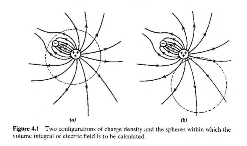
In the first case, all charge is contained within the sphere, so r'<R. Thus we have r_>=R and r_<=r'
This gives us
\int_{r<R}\mathbf{E}(\mathbf{x})\,d^3x=-\frac{R^2}{3\epsilon_0} \int_{}\,d^3x'\frac{ r'}{R^2}\mathbf{n'}\rho(\mathbf{x'})=-\frac{1}{3\epsilon_0}\int_{}r'\frac{\mathbf{x'}}{r'}\rho(\mathbf{x'})\,d^3x' =-\frac{1}{3\epsilon_0}\int_{}\mathbf{x'}\rho(\mathbf{x'})\,d^3x' =-\frac{\mathbf{p}}{3\epsilon_0} where \mathbf{p}=\int_{}\mathbf{x'}\rho(\mathbf{x'})\,d^3x' is the electric dipole moment of the charge distribution with respect to the center of the sphere.
In the second case, since the charge is external to the sphere, we have r'>R. Thus we find
\int_{r<R}\mathbf{E}(\mathbf{x})\,d^3x=-\frac{R^2}{3\epsilon_0} \int_{}\,d^3x'\frac{R}{{r'}^2}\mathbf{n'}\rho(\mathbf{x'})=-\frac{R^3}{3\epsilon_0}\int_{}\,d^3x'\frac{\mathbf{n'}}{{r'}^2}\rho(\mathbf{x'}) =-\frac{R^3}{3\epsilon_0}\int_{}\frac{\mathbf{x'}}{{r'}^3}\rho(\mathbf{x'})\,d^3x'
Now a bit of pattern recognition will prove useful. Notice that this integral is just -4\pi\epsilon_0 times the electric field at the center of the sphere (Coulomb’s Law with \mathbf{x}=\mathbf{0})
Also note that the reason it’s a factor of -4\pi\epsilon_0 and not 4\pi\epsilon_0 is that the integrand here is \frac{\mathbf{x}'-\mathbf{x}}{r^3} instead of \frac{\mathbf{x}-\mathbf{x}'}{r^3} as in Coulomb’s Law.
So we have
\int_{r<R}\mathbf{E}(\mathbf{x})\,d^3x=-\frac{R^3}{3\epsilon_0}\cdot-4\pi\epsilon_0 \mathbf{E}(0)=\frac{4\pi}{3}R^3 \mathbf{E}(0)
Note the sphere’s volumes is \frac{4\pi R^3}{3}
So we have found that the average value of the electric field over a sphere containing no charge equals the field’s value at the sphere’s center. Nice result!
However, returning to the first case, our result there tells us something important.
The traditional expression for the electric field of a dipole at \mathbf{x}_0 is
\mathbf{E}(\mathbf{x})=\frac{3\mathbf{n}(\mathbf{p}\cdot\mathbf{n})-\mathbf{p}}{4\pi\epsilon_0|\mathbf{x}-\mathbf{x}_0|^3}
However, if we integrate this over the volume of the sphere, the resulting integral equals zero. This stands in direct contradiction with our earlier result
\int_{r<R}\mathbf{E}(\mathbf{x})\,d^3x=-\frac{\mathbf{p}}{3\epsilon_0}
To resolve this contradiction, we introduce the Dirac delta function into our formula and write
\mathbf{E}(\mathbf{x})=\frac{1}{4\pi\epsilon_0}\left[\frac{3\mathbf{n}(\mathbf{p}\cdot\mathbf{n})-\mathbf{p}}{|\mathbf{x}-\mathbf{x}_0|^3}-\frac{4\pi}{3}\mathbf{p}\delta(\mathbf{x}-\mathbf{x}_0)\right]
Also note our use of the convention that, when an integral diverges, we consider its limit rather than the nonsensical diverging value. If we didn’t use this convention, the \frac{1}{|\mathbf{x}-\mathbf{x}_0|^3} term would lead to a diverging volume integral.
Now with that convention and the addition of a Dirac delta term, this expression’s volume integral agrees with our previous result.
Thus, through an impressive series of mathematical manipulations, we have found an expression for the dipole’s electric field that removes the contradiction in our earlier expression. And we also found a cool bonus result about the average value of an electric field over a sphere!
Conclusion
This has been a lengthy blog post, so I will briefly summarize our key results.
First, we found a nice bonus result about the average value of an electric field over the surface of a sphere being equal to the field’s value at the sphere’s center.
Then we found our main result. If we integrate the electric field over a sphere containing all charge present in a system, the result will be
\int_{r<R}\mathbf{E}(\mathbf{x})\,d^3x=-\frac{\mathbf{p}}{3\epsilon_0} where \mathbf{p}=\int_{}\mathbf{x'}\rho(\mathbf{x'})\,d^3x' is the electric dipole moment of the charge distribution with respect to the center of the sphere.
We realized that, in order to avoid contradicting this result, we must modify our expression for the electric field casued by a dipole at \mathbf{x}_0
We thus found
\mathbf{E}(\mathbf{x})=\frac{1}{4\pi\epsilon_0}\left[\frac{3\mathbf{n}(\mathbf{p}\cdot\mathbf{n})-\mathbf{p}}{|\mathbf{x}-\mathbf{x}_0|^3}-\frac{4\pi}{3}\mathbf{p}\delta(\mathbf{x}-\mathbf{x}_0)\right]
A number of interesting techniques were used in this derivation. We exploited the expansion in spherical harmonics of \frac{1}{|\mathbf{x}-\mathbf{x'}|} and then made use of the orthogonality of spherical harmonics. We also made good use of many different formulas from electrodynamics, providing a nice example of how different concepts connect at the most unexpected times.
None of the thinking here is greatly original. I merely filled in some missing details in Jackson’s derivation. To anyone interested in seeing more elegant work like this, I highly recommend reading J.D. Jackson’s "Classical Electrodynamics." The book is sometimes difficult to follow, but when you understand him, it feels magical.
I hope that some of the manipulations shown here proved interesting and gave the reader some intellectual satisfaction. As always, if you have any comments or questions, feel free to contact me by email at chancellorceti@gmail.com or on Discord where my username is floofydoggo.
And to anyone reading Jackson’s book, I hope this more detailed derivation has provided more clarity to section 4.1 haha. I spent a few hours this morning understanding that section, so I suppose this is my "April contribution to humanity", if you will. Perhaps this will aid some long-suffering Jackson student.
With all that said, watch for my next blogpost! It will likely involve some more content from Jackson’s monster of a textbook. If you enjoy my writing, be sure to send it to anyone else you think might like it.